Script Tip Friday - How to Plot Stress Gradient Using PyDPF

This Script Tip Friday is brought to you by Ayush Kumar who is a Senior Application Engineer here at Ansys. Ayush will cover how to plot Stress Gradient on a path normal to the selected face at the selected node using PyDPF.

Sometimes for a better engineering decision it is important to analyze results along the normal to a face. This PyDPF example shows you how to plot a stress gradient normal at a selected node on a face.

Import necessary modules: First, import the DPF-Core module as dpf and import the included examples file and DpfPlotter

import matplotlib.pyplot as plt
from ansys.dpf import core as dpf
from ansys.dpf.core import operators as ops
from ansys.dpf.core.plotter import DpfPlotter
from ansys.dpf.core import examples 

Next, link your result file(.rst) and print out the model object. The :class:Model class helps to organize access methods for the result by keeping track of the operators and data sources # used by the result file.

path = r”\Path\to\file.rst"
model = dpf.Model(path)
print(model) 

Define the node_id normal to which a stress gradient should be plotted.

node_id = 1928 

The following command prints the mesh unit

unit = model.metadata.meshed_region.unit
print("Unit: %s" % unit) 

depth defines the path length / depth to which the path will penetrate. While defining depth make sure you use the correct mesh unit. delta defines distance between consecutive points on the path.

depth = 10 # in mm
delta = 0.1 # in mm

Get the meshed region

mesh = model.metadata.meshed_region 

Get Equivalent stress fields container.

stress_fc = model.results.stress().eqv().eval() 

Define Nodal scoping. Make sure to define "Nodal" as the requested location, important for the normals operator.

nodal_scoping = dpf.Scoping(location=dpf.locations.nodal)
nodal_scoping.ids = [node_id] 

Get Skin Mesh because normals operator requires Shells as input.

skin_mesh = ops.mesh.skin(mesh=mesh)
skin_meshed_region = skin_mesh.outputs.mesh.get_data() 

Get normal at a node using normals operator.

normal = ops.geo.normals()
normal.inputs.mesh.connect(skin_meshed_region)
normal.inputs.mesh_scoping.connect(nodal_scoping)
normal_vec_out_field = normal.outputs.field.get_data()

Normal vector is along the surface normal. We need to invert the vector using math.scale operator inwards in the geometry, to get the path direction.

normal_vec_in_field = ops.math.scale(field=normal_vec_out_field, 
                                     ponderation=-1.0)
normal_vec_in = normal_vec_in_field.outputs.field.get_data().data[0]

Get Nodal coordinates, they serve as the first point on the line.

node = mesh.nodes.node_by_id(node_id)
line_fp = node.coordinates 

Create 3D line equation.

fx = lambda t: line_fp[0] + normal_vec_in[0] * t
fy = lambda t: line_fp[1] + normal_vec_in[1] * t
fz = lambda t: line_fp[2] + normal_vec_in[2] * t 

Create coordinates using 3D line equation.

coordinates = [[fx(t * delta), fy(t * delta), fz(t * delta)] for t in range(int(depth / delta))]
flat_coordinates = [entry for data in coordinates for entry in data] 

Create Field for coordinates of the path.

field_coord = dpf.fields_factory.create_3d_vector_field(len(coordinates))
field_coord.data = flat_coordinates
field_coord.scoping.ids = list(range(1, len(coordinates) + 1))  

Let's now map results on the path.

mapping_operator = ops.mapping.on_coordinates(
    fields_container=stress_fc, 
    coordinates=field_coord, 
    create_support=True,
    mesh=mesh
)

fields_mapped = mapping_operator.outputs.fields_container() 

Here, we request the mapped field data and its mesh

field_m = fields_mapped[0]
mesh_m = field_m.meshed_region 

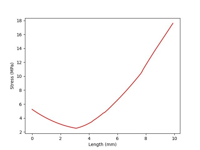
Create stress vs length chart.

x_initial = 0.0
length = [x_initial + delta * index for index in range(len(field_m.data))]
plt.plot(length, field_m.data, "r")
plt.xlabel("Length (%s)" % mesh.unit)
plt.ylabel("Stress (%s)" % field_m.unit)
plt.show() 

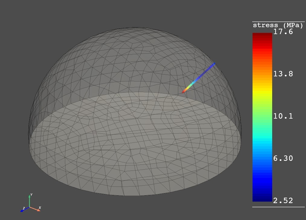
To create a plot, we need to add both the meshes mesh_m - mapped mesh # mesh - original mesh

pl = DpfPlotter()
pl.add_field(field_m, mesh_m)
pl.add_mesh(mesh, style="surface", show_edges=True, 
           color="w", opacity=0.3)
pl.show_figure(show_axes=True, cpos=[ (62.687, 50.119, 67.247), (5.135, 6.458, -0.355), (-0.286, 0.897, -0.336)])