This Script Tip Friday is brought to you by Pernelle Marone-Hitz, Lead Application Engineer at Ansys. Pernelle brings us part 2 of a tip that will cover four examples of Python results for Ansys Mechanical. If you missed Part 1, check it out here.
The Python Result object enables you to evaluate output quantities by executing an Iron-python script based on the Data Processing Framework (DPF) post-processing toolbox.
A previous post showed two examples of Python Results:
- Example 1: Get the maximum over time of the total deformation.
- Example 2: Get the average total deformation on all time steps.
In this new post, we will create four different Python Results of growing complexity.
Example 1: Equivalent Stress
The method here is quite simple, as we will only need to use the dpf.operators.result.stress_von_mises() operator. We simply have to provide the following inputs:
- The data sources: this is simply the result file.
- The time scoping: here we will use the first result set.
The complete script is as follows:
def post_started(sender, analysis):# Do not edit this line
    define_dpf_workflow(analysis)

def define_dpf_workflow(analysis):
    import mech_dpf
    import Ans.DataProcessing as dpf

    my_data_sources = dpf.DataSources(analysis.ResultFileName)
    my_time_scoping = dpf.Scoping()
    my_time_scoping.Ids = [1] # the first set
    s_eqv_op = dpf.operators.result.stress_von_mises()
    s_eqv_op.inputs.requested_location.Connect('Nodal')
    s_eqv_op.inputs.data_sources.Connect(my_data_sources)
    s_eqv_op.inputs.time_scoping.Connect(my_time_scoping)
    dpf_workflow = dpf.Workflow()
    dpf_workflow.Add(s_eqv_op)
    dpf_workflow.SetOutputContour(s_eqv_op)
    dpf_workflow.Record('wf_id', True)
Connect the result:

and then evaluate it. We can then verify that the plot:
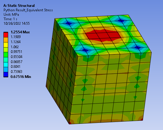
matches the one obtained in a standard Mechanical Equivalent Stress Result:

Example 2: Equivalent Stress on Named Selection
Let’s imagine we have a named selection in the model to identify some specific elements. We’d like to plot the Equivalent Stress again, but only on this Named Selection:
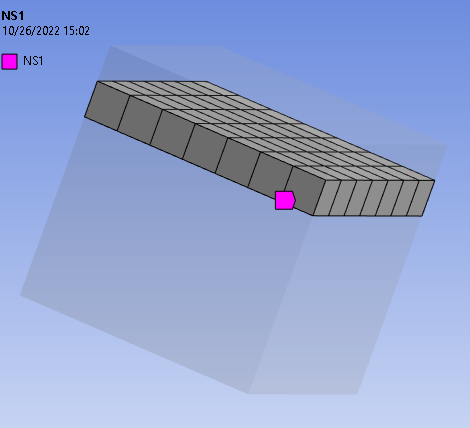
This can be done natively in Mechanical by inserting an Equivalent Stress Result and changing the scoping to the Named Selection:

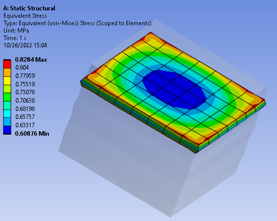
However, we’d like to do the same with a Python Result. The only thing we’ll have to modify from our code in Example 1 is limit the mesh scoping to the nodes in this named selection. This is easily done by adding these two lines of code:
zone1_mesh_region = model.GetNamedSelection('NS1')
s_eqv_op.inputs.mesh_scoping.Connect(zone1_mesh_region)
Note: all named selections defined in Mechanical will be sent to the solver with their names in capital letters. So if a named selection is called ‘my_ns’, the result file will know it as ‘MY_NS’. The complete code is as follows:
def post_started(sender, analysis):# Do not edit this line

    define_dpf_workflow(analysis)

def define_dpf_workflow(analysis):
    import mech_dpf
    import Ans.DataProcessing as dpf

    mech_dpf.setExtAPI(ExtAPI)
    my_data_sources = dpf.DataSources(analysis.ResultFileName)
    model=dpf.Model(my_data_sources)
    my_time_scoping = dpf.Scoping()
    my_time_scoping.Ids = [1] # the first set
    zone1_mesh_region = model.GetNamedSelection('NS1')
    s_eqv_op = dpf.operators.result.stress_von_mises()
    s_eqv_op.inputs.requested_location.Connect('Nodal')
    s_eqv_op.inputs.data_sources.Connect(my_data_sources)
    s_eqv_op.inputs.time_scoping.Connect(my_time_scoping)
    s_eqv_op.inputs.mesh_scoping.Connect(zone1_mesh_region)
    dpf_workflow = dpf.Workflow()
    dpf_workflow.Add(s_eqv_op)
    dpf_workflow.SetOutputContour(s_eqv_op)
    dpf_workflow.Record('wf_id', True)
    this.WorkflowId = dpf_workflow.GetRecordedId()
and this is what we get:
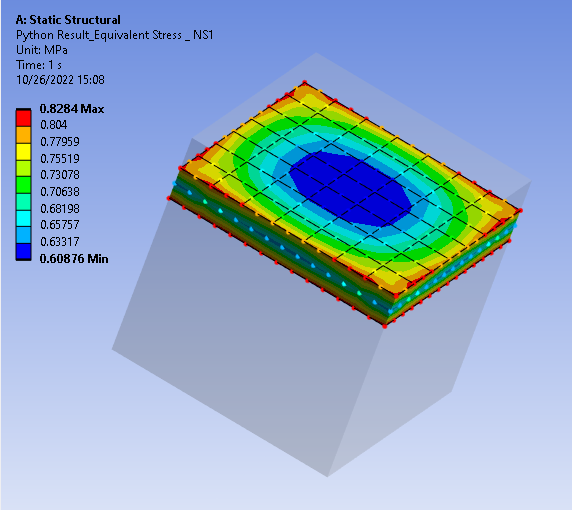
Example 3: Scaled Equivalent Stress on Named Selection
Now we’d like to use the result created in Example 2 but also scale the values by a specified amount. Again, this can be done natively in Mechanical through inserting a User-Defined Result scoped to the Named Selection and with the following expression: SEQV*Val where Val is the scale value.

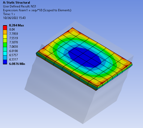
To obtain a similar result through a Python Result, we’ll need two additional things compared to Python Result n°2:
- Use the
math.scale()operator to scale the results - Add a section in the detail’s view of the Python Result so that the user can define the scale value.
Let’s start with the second point. This is done by opening the Property Provider tab and by adding a property as follows:
def reload_props():
    this.PropertyProvider = None

    # Create the property instance
    provider = Provider()
    # Create a group named Group 1.
    group = provider.AddGroup("Group 1")

    # Create a property with control type Expression and a property with control type Double, and add it to the Group 1
    scale_value = group.AddProperty("Scale Value", Control.Double)
    # Connects the provider instance back to the object by setting the PropertyProvider member on this, 'this' being the
    # current instance of the Python Code object.
    this.PropertyProvider = provider
The properties need to be reloaded:

and then we get the line where the scale value can be defined:
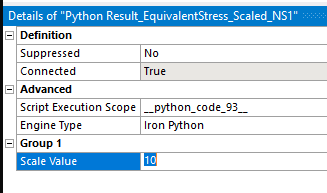
n the script of the Python Code, the value defined as Scale Value can be retrieved by: this.GetCustomPropertyByPath("Group 1/Scale Value").Value
As for the scale operator, we just need to connect it both to the scale value and to the output field of the equivalent stress operator.
The script is as follows:
def post_started(sender, analysis):# Do not edit this line
    define_dpf_workflow(analysis)

def define_dpf_workflow(analysis):
    import mech_dpf
    import Ans.DataProcessing as dpf
    mech_dpf.setExtAPI(ExtAPI)

    my_data_sources = dpf.DataSources(analysis.ResultFileName)
    model=dpf.Model(my_data_sources)
    my_time_scoping = dpf.Scoping()
    my_time_scoping.Ids = [1] # the first set

    zone1_mesh_region = model.GetNamedSelection('NS1')
    s_eqv_op = dpf.operators.result.stress_von_mises()
    s_eqv_op.inputs.requested_location.Connect('Nodal')
    s_eqv_op.inputs.data_sources.Connect(my_data_sources)
    s_eqv_op.inputs.time_scoping.Connect(my_time_scoping)
    s_eqv_op.inputs.mesh_scoping.Connect(zone1_mesh_region)

    scale_value = this.GetCustomPropertyByPath("Group 1/Scale Value").Value
    scale_op = dpf.operators.math.scale()
    scale_op.inputs.field.Connect(s_eqv_op.outputs.fields_container.GetData())
    scale_op.inputs.ponderation.Connect(scale_value)

    dpf_workflow = dpf.Workflow()
    dpf_workflow.Add(scale_op)
    dpf_workflow.SetOutputContour(scale_op)
    dpf_workflow.Record('wf_id', True)
    this.WorkflowId = dpf_workflow.GetRecordedId()
The Python Result can then be evaluated:
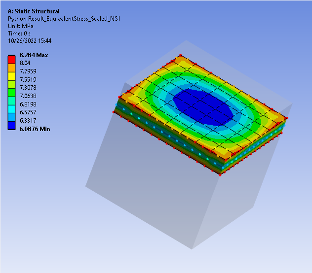
Example 4: Scaled Equivalent Stress on two Named Selections with two different scale values
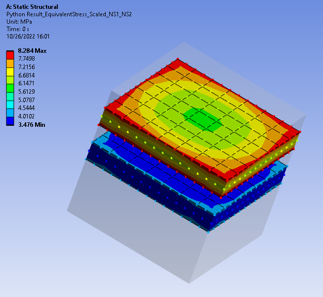
Here we’d like to get on the same plot the following result:
- For nodes belonging to Named Selection n°1, scale the equivalent stress result by value N1.
- For nodes belonging to Named Selection n°2, scale the equivalent stress result by value N2.
This is where we get all the added value of the Python Result object as such a result cannot be obtained in Mechanical. First, we’ll have to change the Property Provider so that the user can input two different scale values (one for NS1, one for NS2). This is easily done by adapting the code created in Example 3:
def reload_props():
    this.PropertyProvider = None

    """

    Some sample code is provided below that shows how to:

        1. Create an instance of the Provider. The Provider class is used to add custom properties to the details.

        2. Use the Provider instance to add custom properties.

        3. Configure those custom properties.

    """
    # Create the property instance
    provider = Provider()

    # Create a group named Group 1.
    group = provider.AddGroup("Group 1")
 n   # Create a property with control type Expression and a property with control type Double, and add it to the Group 1

    scale_foam1 = group.AddProperty("Scale Value 1", Control.Double)
    scale_foam2 = group.AddProperty("Scale Value 2", Control.Double)

    # Configure the double property to be parameterizable. As a default the property will be an input parameter.
    # However, by updating the ParameterType property, it can be configured to be a output parameter as well.
    # double_prop.CanParameterize = True
    # double_prop.ParameterType = ParameterType.Output

    # Connects the provider instance back to the object by setting the PropertyProvider member on this, 'this' being the
    # current instance of the Python Code object.
    this.PropertyProvider = provider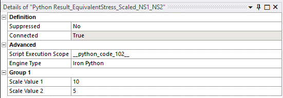
The code created for Example 3 is easily adapted so that we get two output fields:
- Scaled stress for NS1
- Scaled stress for NS2.
The only remaining task is to combine both fields into a unique field so that the result can be plotted on the model. The dpf.operators.utility.merge_fields_containers() operator is the operator we need for that. The complete code is as follows:
def post_started(sender, analysis):  # Do not edit this line
    define_dpf_workflow(analysis)

def define_dpf_workflow(analysis):
    import mech_dpf
    import Ans.DataProcessing as dpf

    mech_dpf.setExtAPI(ExtAPI)
    my_data_sources = dpf.DataSources(analysis.ResultFileName)
    model = dpf.Model(my_data_sources)
    scale_zone1 = this.GetCustomPropertyByPath("Group 1/Scale Value 1").Value
    scale_zone2 = this.GetCustomPropertyByPath("Group 1/Scale Value 2").Value

    # Read mesh in results fil
    mesh_op = dpf.operators.mesh.mesh_provider()  # operator instanciation
    mesh_op.inputs.data_sources.Connect(my_data_sources)
    mesh = mesh_op.outputs.mesh.GetData()
    # Define time scoping
    my_time_scoping = dpf.Scoping()
    my_time_scoping.Ids = [1]  # the first set

    # Get named selection
    zone1_mesh_region = model.GetNamedSelection('NS1')
    zone2_mesh_region = model.GetNamedSelection('NS2')

    # Get equivalent stresses on named selections
    s_eqv_op_zone1 = dpf.operators.result.stress_von_mises()
    s_eqv_op_zone1.inputs.requested_location.Connect('Nodal')
    s_eqv_op_zone1.inputs.data_sources.Connect(my_data_sources)
    s_eqv_op_zone1.inputs.time_scoping.Connect(my_time_scoping)
    s_eqv_op_zone1.inputs.mesh_scoping.Connect(zone1_mesh_region)
    s_eqv_op_zone2 = dpf.operators.result.stress_von_mises()
    s_eqv_op_zone2.inputs.requested_location.Connect('Nodal')
    s_eqv_op_zone2.inputs.data_sources.Connect(my_data_sources)
    s_eqv_op_zone2.inputs.time_scoping.Connect(my_time_scoping)
    s_eqv_op_zone2.inputs.mesh_scoping.Connect(zone2_mesh_region)

    # Scale results
    scale_op_zone1 = dpf.operators.math.scale_fc()
    scale_op_zone1.inputs.fields_container.Connect(
        s_eqv_op_zone1.outputs.fields_container.GetData())
    scale_op_zone1.inputs.ponderation.Connect(scale_zone1)
    scale_op_zone1_fc = scale_op_zone1.outputs.fields_container
    scale_op_zone2 = dpf.operators.math.scale_fc()
    scale_op_zone2.inputs.fields_container.Connect(
        s_eqv_op_zone2.outputs.fields_container.GetData())
    scale_op_zone2.inputs.ponderation.Connect(scale_zone2)
    scale_op_zone2_fc = scale_op_zone2.outputs.fields_container

    # Create combined result
    op = dpf.operators.utility.merge_fields_containers()  # operator instantiation
    op.inputs.fields_containers1.Connect(scale_op_zone1_fc)
    op.inputs.fields_containers2.Connect(scale_op_zone2_fc)
    my_merged_fields_container = op.outputs.merged_fields_container
    combined_plot = dpf.operators.utility.forward_field()  # operator instanciation
    combined_plot.inputs.field.Connect(my_merged_fields_container)
    dpf_workflow = dpf.Workflow()
    dpf_workflow.Add(combined_plot)
    dpf_workflow.SetOutputContour(combined_plot,
                                  dpf.enums.GFXContourType.FENodalScoping)
    dpf_workflow.Record('wf_id', True)
    this.WorkflowId = dpf_workflow.GetRecordedId()
The result then can be evaluated:
