Turbomachinery application: A comprehensive inverse-solving (hot-to-cold) simulation workflow using PyAnsys libraries to analyze the NASA Rotor 67 fan-bladed disk

Introduction

In recent years, the aerospace and turbomachinery industries have experienced remarkable progress in the design and development of high-performance, efficient turbomachinery components. Rotor fans and disks, which serve as critical components in propulsion systems and energy conversion devices, significantly impact the overall efficiency and reliability of these advanced machines.

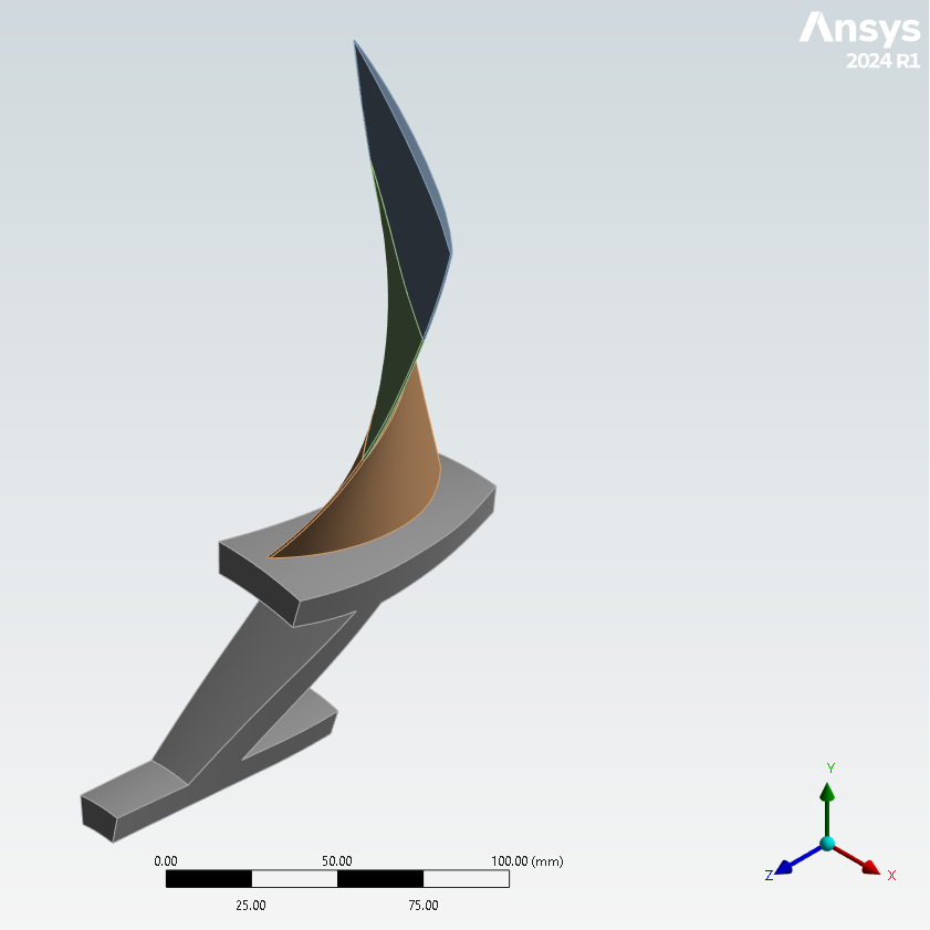
Within this context, the NASA Rotor 67 fan-bladed disk is a subsystem of a turbofan compressor set employed in aerospace engine applications. This sector model, which exemplifies a challenging industrial case with publicly available detailed geometry and flow information, comprises a disk and fan blade with a sector angle of 16.364 degrees. The sector model embodies the blade's running or hot geometry, and it is already optimized for running conditions under loading. The primary objective of the proposed simulation workflow involves deriving the cold geometry (for manufacturing) from the provided hot geometry through inverse solving.

Note: In turbomachinery engineering, the hot-to-cold method is a prevalent approach for designing rotor blades. The rotor blade geometry representing the as-manufactured shape is referred to as the cold geometry, while the shape of the rotor blade during running conditions is known as the hot geometry.

Overview

This blog introduces a comprehensive, inverse-solving (hot-to-cold) simulation workflow using PyAnsys libraries to analyze the NASA Rotor 67 fan-bladed disk. PyAnsys libraries are versatile Python libraries that effectively integrate with Ansys engineering simulation tools to facilitate efficient, automated processes. The blog showcases how to streamline Mechanical simulations with PyMechanical, postprocess results with PyDPF-Post, and generate detailed reports with PyDynamicReporting. By leveraging these PyAnsys libraries, the proposed workflow delivers a potent solution for designing and innovating next-generation rotor fan-bladed disks, ultimately driving advancements in turbomachinery applications.

The primary focus of this document is to provide a step-by-step guide to simulating an inverse (hot-to-cold) process using PyMechanical. To gain an introductory understanding of the installation, setup, and advanced features of PyMechanical, including an in-depth example, see the latest release of the PyMechanical documentation.

Additionally, this blog explores the capabilities of the Python client library for the Data Processing Framework (DPF), known as PyDPF-Post. This PyAnsys library is specifically designed for postprocessing simulation results, enabling you to analyze and visualize data effectively. For comprehensive information on PyDPF-Post, including detailed documentation and step-by-step installation instructions, see the latest release of the PyDPF-Post documentation.

The final section of this blog demonstrates how to use PyDynamicReporting to access and integrate generated reports with modern technology stacks, facilitating a smooth integration into end-to-end workflows. This allows you to maximize the efficiency of your simulation processes and leverage cutting-edge tools for data analysis and visualization. For a deeper understanding of these features and guidance on installation, see the latest release of the PyDynamicReporting documentation.

By the time you reach the end of this blog, you will have a thorough understanding of PyMechanical's capabilities and how to harness its power for simulating complex processes. Furthermore, you will be well-equipped to use PyDPF-Post for postprocessing simulation results and PyDynamicReporting for seamlessly incorporating generated reports into contemporary technology stacks, thereby optimizing your workflow and enhancing productivity.

Set up your environment

Before you can use PyAnsys libraries, you must set up your environment. First, ensure that you have legally licensed copies of these Ansys products installed:

Once these Ansys products are installed, set up your environment:

Install Python (if not already installed).

Ensure that you have Python installed on your system. You can download Python from the official website. The recommended version is Python 3.10.
Create a virtual environment (if not already created).
```
  python -m venv .venv      
```
Activate the virtual environment.
- For Windows CMD:
```
  .venv\Scripts\activate.bat
```
- For Windows Powershell:
```
  .venv\Scripts\Activate.ps1
```
- For Linux:
```
  source .venv/bin/activate
```
From this point forward, you must execute all commands within the virtual environment.
Install the libraries.

Now that your virtual environment is active, you can use pip to install the required PyAnsys libraries. Run the following commands to install the ansys-mechanical-core, ansys-dpf-core, ansys-dpf-post, and ansys-dynamicreporting-core packages:
```
pip install ansys-mechanical-core
pip install ansys-dpf-core
pip install ansys-dpf-post
pip install ansys-dynamicreporting-core
```

Note: For beginners who find the preceding steps challenging, consider using the Ansys Python Manager to install Python and PyAnsys metapackages. This tool also simplifies the process of creating and managing virtual environments.

Use PyMechanical to simulate the inverse-solving (hot-to-cold) workflow

To familiarize yourself with the PyMechanical scripting interface, first see Exploring PyMechanical access methods: A brief overview on the Ansys Developer Portal. Then, return to this blog to delve into the following key features of PyMechanical:

Import a geometry from a supported CAD file using the Import Geometry option.
Import a material database by reading a XML file format using the Import Material option.
Import a CFX generated pressure and temperature data from external source files directly into the application using an External Data system.

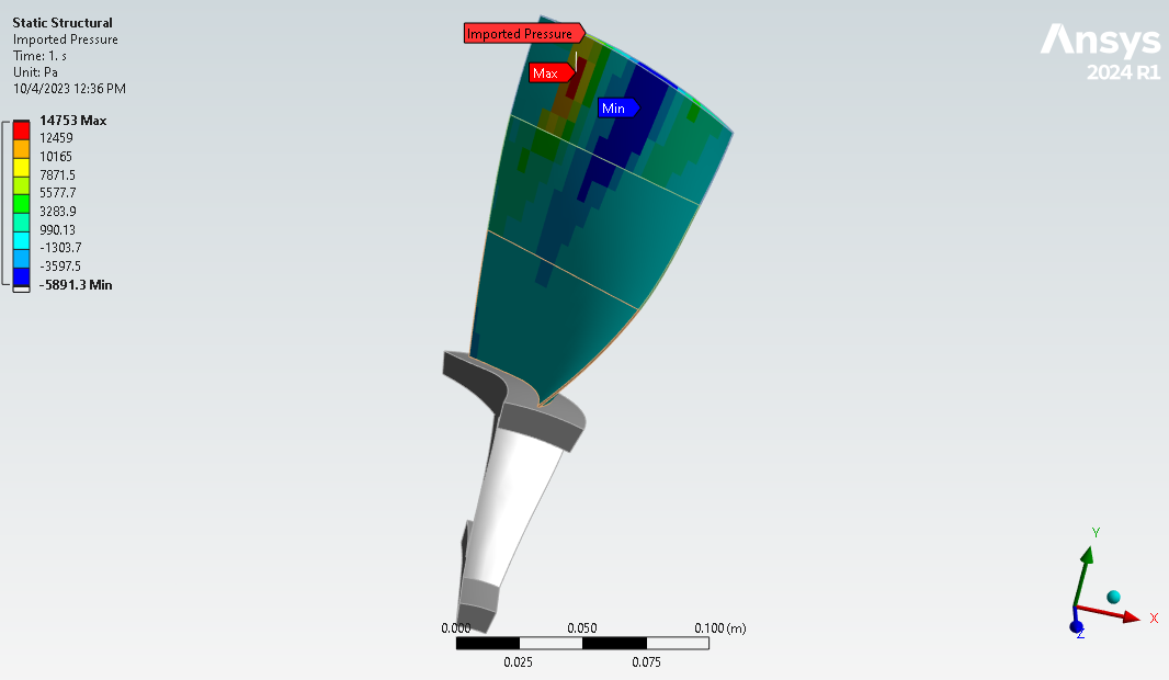
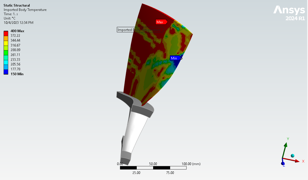
During the simulation process for any mechanical application, a series of standard steps are followed for modeling, which include importing the geometry and the materials. In terms of loading, a rotational velocity (CGOMGA,0,0,1680) is applied along the global Z-axis. The reference temperature is consistently maintained at 22 degrees Celsius, while temperature loading is implemented on the blade (BF). Furthermore, unsteady flow pressures (imported from Ansys CFX) are produced for an engine-order excitation of EO=2 at a rotational frequency of 534.76 Hz. This pressure data is subsequently mapped to the structural rotor fan blade model in the Mechanical application using an External Data system.

Simulate the gas turbine-focused workflow

Import required libraries and modules.

import ansys.mechanical.core as mech
from ansys.mechanical.core.examples import delete_downloads, download_file
from Ansys.ACT.Interfaces.Common import *
from Ansys.ACT.Mechanical.Fields import *
from Ansys.Mechanical.DataModel.Enums import *
from Ansys.Mechanical.DataModel.MechanicalEnums import *

Download geometry (.agdb/.pmdb) file.

geometry_path = download_file(
    "example_10_td_055_Rotor_Blade_Geom.pmdb", "pymechanical", "embedding"
)

*Download material (.xml) file.**

mat_path = download_file(
    "example_10_td_055_Rotor_Blade_Mat_File.xml", "pymechanical", "embedding"
)

*Download CFX pressure (.csv) file.**

cfx_data_path = download_file(
    "example_10_CFX_ExportResults_FT_10P_EO2.csv", "pymechanical", "embedding"
)

*Download CFX temperature (.txt) file.**

temp_data_path = download_file(
    "example_10_Temperature_Data.txt", "pymechanical", "embedding"
)

Launch an embedded Mechanical session.

app = mech.App(version=241)
globals().update(mech.global_variables(app, True))
print(app)

Import the geometry file into the application.

geometry_import_group = Model.GeometryImportGroup
geometry_import = geometry_import_group.AddGeometryImport()
geometry_import_format = (
    Ansys.Mechanical.DataModel.Enums.GeometryImportPreference.Format.Automatic
)
geometry_import_preferences = Ansys.ACT.Mechanical.Utilities.GeometryImportPreferences()
geometry_import_preferences.ProcessNamedSelections = True
geometry_import_preferences.NamedSelectionKey = ""
geometry_import_preferences.ProcessMaterialProperties = True
geometry_import_preferences.ProcessCoordinateSystems = True
geometry_import.Import(
    geometry_path, geometry_import_format, geometry_import_preferences
)

Import the material file into the application.

materials = ExtAPI.DataModel.Project.Model.Materials
materials.Import(mat_path)

Import CFX-generated pressure data into the application.

Imported_Load_Group = STAT_STRUC.AddImportedLoadExternalData()

external_data_files = Ansys.Mechanical.ExternalData.ExternalDataFileCollection()
external_data_files.SaveFilesWithProject = False
external_data_file_1 = Ansys.Mechanical.ExternalData.ExternalDataFile()
external_data_files.Add(external_data_file_1)
external_data_file_1.Identifier = "File1"
external_data_file_1.Description = ""
external_data_file_1.IsMainFile = False
external_data_file_1.FilePath = cfx_data_path
external_data_file_1.ImportSettings = (
    Ansys.Mechanical.ExternalData.ImportSettingsFactory.GetSettingsForFormat(
        Ansys.Mechanical.DataModel.MechanicalEnums.ExternalData.ImportFormat.Delimited
    )
)
import_settings = external_data_file_1.ImportSettings
import_settings.SkipRows = 17
import_settings.SkipFooter = 0
import_settings.Delimiter = ","
import_settings.AverageCornerNodesToMidsideNodes = False
import_settings.UseColumn(
    0,
    Ansys.Mechanical.DataModel.MechanicalEnums.ExternalData.VariableType.XCoordinate,
    "m",
    "X Coordinate@A",
)
import_settings.UseColumn(
    1,
    Ansys.Mechanical.DataModel.MechanicalEnums.ExternalData.VariableType.YCoordinate,
    "m",
    "Y Coordinate@B",
)
import_settings.UseColumn(
    2,
    Ansys.Mechanical.DataModel.MechanicalEnums.ExternalData.VariableType.ZCoordinate,
    "m",
    "Z Coordinate@C",
)
import_settings.UseColumn(
    3,
    Ansys.Mechanical.DataModel.MechanicalEnums.ExternalData.VariableType.Pressure,
    "Pa",
    "Pressure@D",
)

Imported_Load_Group.ImportExternalDataFiles(external_data_files)
Imported_Pressure = Imported_Load_Group.AddImportedPressure()
selection = NS_GRP.Children[2]
Imported_Pressure.Location = selection

pressure_id = Imported_Pressure.ObjectId
Imported_Pressure = ExtAPI.DataModel.GetObjectById(pressure_id)
Imported_Pressure.AppliedBy = LoadAppliedBy.Direct
Imported_Pressure.ImportLoad()

Import CFX-generated temperature data into the application.

Imported_Load_Group = STAT_STRUC.AddImportedLoadExternalData()

external_data_files = Ansys.Mechanical.ExternalData.ExternalDataFileCollection()
external_data_files.SaveFilesWithProject = False
external_data_file_1 = Ansys.Mechanical.ExternalData.ExternalDataFile()
external_data_files.Add(external_data_file_1)
external_data_file_1.Identifier = "File1"
external_data_file_1.Description = ""
external_data_file_1.IsMainFile = False
external_data_file_1.FilePath = temp_data_path

external_data_file_1.ImportSettings = (
    Ansys.Mechanical.ExternalData.ImportSettingsFactory.GetSettingsForFormat(
        Ansys.Mechanical.DataModel.MechanicalEnums.ExternalData.ImportFormat.Delimited
    )
)
import_settings = external_data_file_1.ImportSettings
import_settings.SkipRows = 0
import_settings.SkipFooter = 0
import_settings.Delimiter = ","
import_settings.AverageCornerNodesToMidsideNodes = False
import_settings.UseColumn(
    0,
    Ansys.Mechanical.DataModel.MechanicalEnums.ExternalData.VariableType.XCoordinate,
    "m",
    "X Coordinate@A",
)
import_settings.UseColumn(
    1,
    Ansys.Mechanical.DataModel.MechanicalEnums.ExternalData.VariableType.YCoordinate,
    "m",
    "Y Coordinate@B",
)
import_settings.UseColumn(
    2,
    Ansys.Mechanical.DataModel.MechanicalEnums.ExternalData.VariableType.ZCoordinate,
    "m",
    "Z Coordinate@C",
)
import_settings.UseColumn(
    3,
    Ansys.Mechanical.DataModel.MechanicalEnums.ExternalData.VariableType.Temperature,
    "C",
    "Temperature@D",
)

Imported_Load_Group.ImportExternalDataFiles(external_data_files)
imported_body_temperature = Imported_Load_Group.AddImportedBodyTemperature()

selection = NS_GRP.Children[1]
imported_body_temperature.Location = selection
imported_load_id = imported_body_temperature.ObjectId
imported_load = DataModel.GetObjectById(imported_load_id)
imported_load.ImportLoad()

Save the project and clean up the Ansys Mechanical session.

app.save(os.path.join(cwd, "blade_inverse.mechdat"))
app.new()

The preceding steps describe the process of accessing simulation data and initiating an embedded Ansys Mechanical session using PyMechanical. This includes importing geometry and material files. These steps also demonstrate mapping of CFX-generated pressure and temperature data imported via an External Data system. The subsequent sections guide you through using PyDPF-Post for postprocessing results and PyDynamicReporting for generating reports.

Use PyDPF-Post to postprocess results

To postprocess the results from the inverse-solving simulation, you use PyDPF-Post. This blog describes how to use these PyDPF-Post features:

Postprocess result quantities using physics-oriented APIs, which enable auto-completion.
Compute the minimum and maximum of a dataframe, which are generated by extracting a result from a simulation.

Postprocess results from the gas turbine-focused workflow

Import required libraries and modules.

from ansys.dpf import post
from ansys.dpf.post import examples

Get the Simulation object.

Get the Simulation object that allows access to the results. The Simulation object must be instantiated with the path for the result file. For example, "C:/Users/user/my_result.rst" on Windows or "/home/user/my_result.rst"on Linux.

example_path = examples.download_inversesolve()
simulation = post.StaticMechanicalSimulation(example_path)
print(simulation)

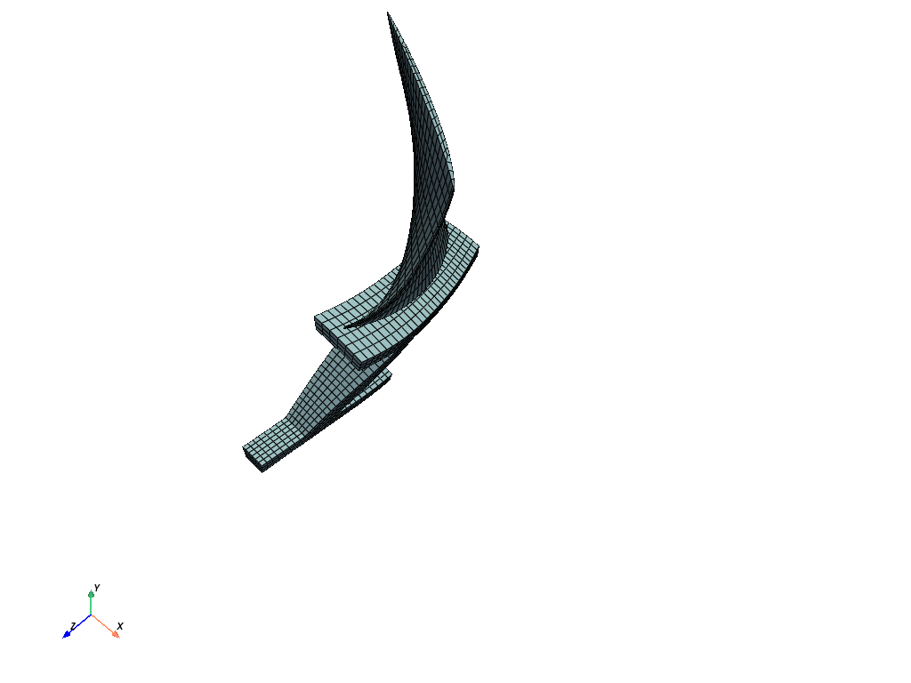
Get the mesh from the Simulation object.

mesh = simulation.mesh
mesh.plot(title="Element Plot",screenshot="mesh.png",off_screen=True, cpos=cpos)

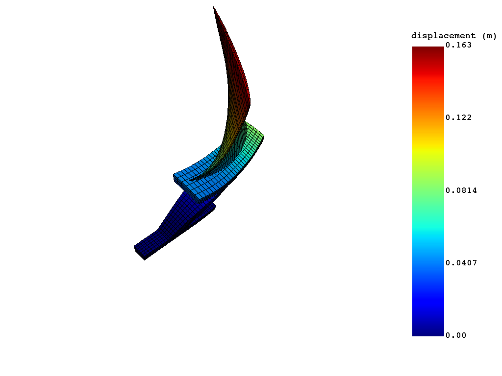
Compute total displacement quantities.

displacement = simulation.displacement(set_ids=[10])
displacement.plot(title="Total displacement",screenshot="tot_deform_1.png",off_screen=True, cpos=cpos)

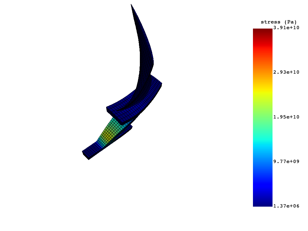
Compute nodal equivalent stress quantities.

eqv_stress = simulation.stress_eqv_von_mises_nodal(set_ids=[10])
eqv_stress.plot(title="Nodal Equivalent Stress",screenshot="eqv_stress_4.png",off_screen=True, cpos=cpos)

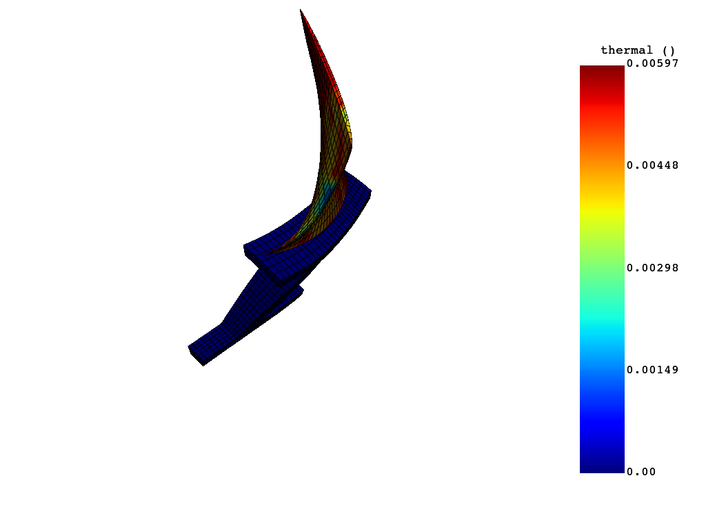
Compute nodal thermal strain quantities.

nodal_thermal_strain = simulation.thermal_strain_nodal(components=["XX"],load_steps=(1,10))
nodal_thermal_strain.plot(title="Nodal Thermal Strain",screenshot="eqv_thermal_Strain_6.png",off_screen=True, cpos=cpos)

![Strain visualization]https://developer.ansys.com/sites/default/files/inline-images/eqv_thermal_Strain_6.png)

The preceding steps show how to use PyDPF to postprocess the simulation results. The subsequent section shows how to use PyDynamicReporting for report generation.

Use PyDynamicReporting to create Ansys reports

To create Ansys reports from the result images postprocessed by PyDPF-Post, you use PyDynamicReporting. Key features of PyDnamicReporting include:

Native support for multiple data formats
Ability to store data from various sources, such as CAD packages, simulation software, and postprocessors
Tools for data aggregation, filtering, and processing within the database
A web-based interface for seamless and intuitive interaction with database items

Connect to the Ansys Dynamic Reporting (ADR) server

Import required libraries and modules.

from pathlib import Path
import ansys.dynamicreporting.core as adr

Start the ADR server as a service.

ansys_loc = r'C:\Program Files\ANSYS Inc\v241'
adr_service = adr.Service(ansys_installation = ansys_loc, db_directory = new_dir)
session_guid = adr_service.start(create_db = True)

Create an Ansys report from a template.

You can create an Ansys report from a template, modifying it as per your requirements.

# Create items
my_text = adr_service.create_item()
my_text.item_text = "<h2>Inverse-solving analysis (hot-to-cold) of a rotor fan-bladed disk</h2>"
my_text = adr_service.create_item()
my_text.item_text = "<p>In turbomachinery engineering, the hot-to-cold method is commonly used to design rotor blades. \
    The rotor blade geometry that would represent the as-manufactured shape is referred to as the cold geometry, whereas \
    the shape of the rotor blade in the running condition is referred to as the hot geometry.</p>"
my_text = adr_service.create_item()
my_text.item_text = "<h3>Introduction</h3>The NASA Rotor 67 fan-bladed disk is a subsystem of a turbofan compressor \
    set used in aerospace engine applications. This sector model, representing a challenging industrial example for which \
    the detailed geometry and flow information is available in the public domain, consists of a disk and a fan blade with \
    a sector angle of 16.364 degrees. The sector model represents the running condition or hot geometry of the blade. It is \
    already optimized at the running condition under loading. The primary objective is to obtain the cold geometry \
    (for manufacturing) from the given hot geometry using inverse solving."

# Create tables and trees
my_text = adr_service.create_item()
my_text.item_text = "<h4><br>Material properties</br></h4>The model uses linear elastic material. \
    The following temperature-dependent material properties are used:"
my_text = adr_service.create_item()
my_text.item_text = "<p><b><br>Material properties for the NASA Rotor 67 fan-bladed disk</br></b></p>"

my_plot = adr_service.create_item()
my_plot.item_table = np.array([[22, 200, 300, 600], [2.2E11, 2.0E11, 1.9E11, 1.8E11], \
                               [0.27,0.28, 0.29, 0.30],[7840, 7740, 7640, 7540],[1.2E-5, 1.3E-5, 1.4E-5, 1.5E-5]], dtype="|S20")
my_plot.labels_row = ["Temperature (C)", "Young's Modulus (Pa)","Poisson's Ratio","Density (kg/m^3)","Coefficient of Thermal Expansion"]

my_text = adr_service.create_item()
my_text.item_text = "<p><b><br>End of the report</br></b></p>"

# Create the report template
template_0 = adr_service.serverobj.create_template(name="MyReport", parent=None, report_type="Layout:basic")
template_0.params = '{"properties": {"item_justification": "left"}}'
adr_service.serverobj.put_objects(template_0)

# Visualize the report "MyReport"
adr_service.visualize_report(report_name = "MyReport")

Close the ADR service.

adr_service.stop()

Conclusion

The comprehensive ecosystem of PyAnsys libraries serves as an indispensable asset for engineers and researchers involved in gas turbine-centric workflows. By seamlessly integrating powerful tools such as Ansys Mechanical, Ansys DPF, Ansys Dynamic Reporting, and their corresponding Python client libraries--PyMechanical, PyDPF-Post, and PyDynamicReporting, you can significantly streamline simulation and reporting procedures. Moreover, these tools provide you with a plethora of application and integration possibilities that cater to a wide range of use cases.

In this rapidly evolving, technology-driven landscape, these cutting-edge tools empower you to fully harness the potential of your simulation data. By doing so, you are able to drive innovation, enhance decision-making, and ultimately optimize performance in the realm of gas turbine technology. Overall, PyAnsys libraries are a testament to the synergy of advanced software and engineering expertise, paving the way for continued progress in this critical industry.