This article is brought to you by Sotirios Kakaletsis. You can find out more about his research on his website and contact him via his LinkedIn.
Introduction
In this article, we explore the mechanical behavior of a flexible, biomedical catheter under large deformation. Using the scripting capabilities of PyMAPDL, we perform an iterative analysis to evaluate the apparent flexural rigidity of the catheter under different design configurations.
The Catheter
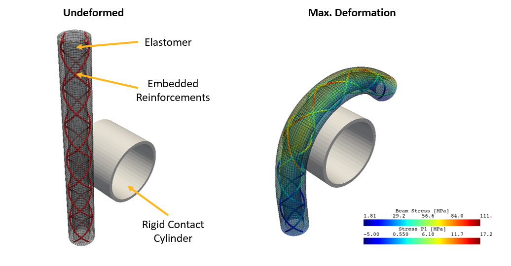
We model a braided biomedical catheter as a reinforced elastomer. For the elastomer we use the incompressible neo-Hookean (rubber-like) material model, whereas the reinforcements are much stiffer, linear elastic beams.
Through embedding stiff reinforcements we aim to achieve the required axial, flexural and torsional rigidity, as described -for example- in the case of cardiovascular catheters (J. Carey et al., 2004).
Within the scope of this example, we will focus on the apparent flexural rigidity measured as the reaction bending moment of the catheter, while it wraps around a rigid cylinder (see following figure).
The Pipeline
Via a main script and for each set of design parameters, we iteratively call the function Run_Catheter() that formulates the MAPDL model and runs the corresponding simulation. Once the run is complete, we call the post processing scripts Plotter() and Animator() to visualize the stress fields of the elastomer and the reinforcing beams.

Step 1: Define basic model input
We first define the basic model input parameters, such as the dimensions, the boundary conditions and the design parameters to be explored. In this case, we focus on the coil angles, expressed as the number of complete loops the reinforcements form over the length of the catheter.
# Basic Model Input
mdl_name = 'HelixAngleStudy'
Ra = 0.6 # Inner Radius
Rb = 0.9 # Outer Radius
Rm = (Ra+Rb)/2 # Coil Radius
H  = 15 # Height of catheter
n_cables = 4 # Number of coil-reinforcements
hs = 0.15 # Solid Element length
hb = 0.20 # Beam Element length

# Define Boundary Conditions
ActiveBCs = {'UxAct':False, 'UyAct':False, 'UzAct':False, 'RxAct':True, 'RyAct':True, 'RzAct':True}
BoundaryCond = {'Ux':0, 'Uy':0.0, 'Uz':0, 'Rx':0 , 'Ry': 1.5*np.pi/2,'Rz':0}
BoundaryCond.update(ActiveBCs)

# Full loops for each coil-reinforcement
helix_angles = np.array([1,2,3,4,5,6,7])*2*np.pi
Step 2: Perform the analysis
In the main script again and following the definition of the input, we initialize the MAPDL session. Next, for each value of helix angle, we perform a simulation of the bending problem. The output and the quantity of interest in this case is the reaction bending moment as a function of the prescribed, rotation angle.
# Initialize MAPDL
path = os.getcwd() # Get current working directory
path = path +'/'+mdl_name
isExist = os.path.exists(path)
if not isExist:
   # Create a new directory because it does not exist
   os.makedirs(path)
mapdl = pymapdl.launch_mapdl(run_location=path, nproc=6)

# Helix Angle Study
TotUF = [] # Reaction forces & Displacements
for idx, helix_angle in enumerate(helix_angles):
    fl_name = mdl_name + str(idx)
    U_F_ = Run_Catheter(mapdl,fl_name,Ra, Rb, Rm, H, n_cables, helix_angle, sol_el_size=hs, beam_el_size=hb, BCs = BoundaryCond)
    U_F_['CoilAngle'] = helix_angle
    U_F_['n_cables'] = n_cables
    TotUF.append(U_F_)

    #Save in each iteration, just in case
    f = open('./' + mdl_name + '.pkl', 'wb')
    pickle.dump([hs, hb, TotUF], f)

mapdl.exit()
Intermediate steps: Building the model
As we mentioned previously, within our framework, the main script calls the function Run_Catheter() which builds and runs each simulation, separately.
As a first step, we define the two material types, one for the elastomer and another for the reinforcements.
#--------------- MATERIALS---------------------------
# Define Base material
D1 = 1 / (C10 * k_mu_ratio)  # for nearly incompressible neo-hookean
mapdl.tb('HYPER', mat=1, tbopt='NEO')
mapdl.tbdata(stloc=1, c1=C10, c2=D1)

# Define Beam material
mapdl.mp("EX", 2, Eb)  # Elastic modulus
mapdl.mp("DENS", 2, 7800)  # Density in kg/m3
mapdl.mp("NUXY", 2, beam_nu)  # Poisson's Ratio
In the same function, next we define the various solid geometries, (cylinders), and the corresponding contact surfaces. Note, that this process involves defining local coordinate (cylindrical) systems, to accommodate for the different solid orientation, as follows:
#-------------- GEOMETRY -----------------------------
# Create Elastomer Cylinder
vnum0 = mapdl.cylind(Ra, Rb, 0, H)
mapdl.et(1, 185, kop2=0, kop6=1)  # SOLID185 C3D8H
mapdl.esize(sol_el_size)
mapdl.type(1)  # Sets type1 to subsequent meshing scheme
mapdl.mat(1)  # Set the material to neo-Hookean
mapdl.vsweep(vnum0)

# Define Contact Elements
mapdl.starset('cid',3)
mapdl.r('cid')
mapdl.real('cid')
mapdl.et('cid', 174)
mapdl.seltol(1e-12)
mapdl.local(10000, 1)
mapdl.nsel('S','LOC','X', Rb)
mapdl.type('cid')
mapdl.esurf()

# Create Contact Cylinder (Rigid)
Rcyl = 2.5* Rb
Lcyl = 4 * Rb
XC = (Rb + Rcyl)
YC= -0.5 * Lcyl
ZC = H / 3
mapdl.wplane(-1, XC, YC, ZC, 2 * XC, YC, ZC, XC, YC, 0)
mapdl.csys(4) # Change coordinate system to  global one
vnum1 = mapdl.cylind(0.9*Rcyl, Rcyl, 0, Lcyl)
mapdl.et(10, 185, kop2=0)  # SOLID185 C3D8H
mapdl.esize(0.25)
mapdl.type(10)  # Sets type1 to subsequent meshing scheme
mapdl.mat(1)    # Set the material to neo-Hookean
mapdl.vsweep(vnum1)
mapdl.wpcsys(-1, 0)
mapdl.csys(0)

# Define local coordinate system to define contact surface
mapdl.starset('tid', 4)
mapdl.r('tid')
mapdl.et('tid', 170)
mapdl.local(1000, 1, XC, YC, ZC, 0, 90, 0)
mapdl.nsel('S','LOC',"X", Rcyl)
mapdl.type('tid')
mapdl.esurf()
mapdl.local(1, 0)
mapdl.csys(0)
Next, we analytically define the topology of the reinforcements, using the general formula x = cos t, y = sin t, z = t, where t is the curve parameter, by generating keypoints and lines on the helical domain.
for i in range(0, n_to_iter):
    ang_offest = n_on_radi[i]
    if (i%2)==0:
        coil_dir = 1
    else:
        coil_dir = -1
    for x in helix_pnts:
        cnt = cnt + 1
        mapdl.k(1000 + cnt, Rm * np.cos(coil_dir*x+ang_offest),  Rm * np.sin(coil_dir*x+ang_offest),  c * x)
Subsequently, we issue the eembed command to embed the beam elements in to the solid domain
# Create reinfocement ellements
mapdl.esel('all')
mapdl.run("eembed")
Within the Run_Catheter() function we also define the boundary conditions, at the free end of the catheter using a remote point rigid constraint.
# Right Edge
mapdl.type('cid')
mapdl.real('cid')
mapdl.nsel("S", "LOC", "Z", H)
mapdl.esurf()
mapdl.seltol() #Set to default

# CreateTarget elements
mapdl.type('tid')
mapdl.mat('cid')
mapdl.real('cid')
mapdl.tshap('pilo')
IDn = mapdl.n('', x=0, y=0, z=H)
mapdl.en(999999, IDn)
mapdl.tshap()

#------ BCs: Rigid displacement on the other end -------------
if BCs['UxAct']:
    mapdl.d(IDn, "UX", BCs['Ux'])
if BCs['UyAct']:
    mapdl.d(IDn, "Uy", BCs['Uy'])
if BCs['UzAct']:
    mapdl.d(IDn, "UZ", BCs['Uz'])
if BCs['RxAct']:
    mapdl.d(IDn, "ROTX", BCs['Rx'])
if BCs['RyAct']:
    mapdl.d(IDn, "ROTY",  BCs['Ry'])
if BCs['RzAct']:
    mapdl.d(IDn, "ROTZ",  BCs['Rz'])
The next intermediate steps in the same function include setting up and calling standard MAPDL solver commands.
For the last step of this script, we visualize the stress fields of the solid domain, using the PyVista library, in the C_Plotter() function. An important point here is to render the 3D beam profiles as tubes, using the respective function.
# Apply the tube filter to beams
pl.update_coordinates(xyz['beam'], mesh=BeamGrid)
beam_grid_srf = BeamGrid.extract_surface()
beam_line = beam_grid_srf.tube(radius=beam_radius)
pl.add_mesh(beam_line, scalar_bar_args=sargs)
Summary and Outlook
The next figure summarizes the findings of our analysis. Our pipeline identifies a range of helix coil angle (or equivalently, the coil pitch) for which the reaction bending moment is minimized. Following the same procedure, the PyMADPL user can optimize other features as well, including stiffness ratio, reinforcement density, various materials.
Overall, the PyMADL framework provides the user with many powerful tools, such as incorporating external libraries, run scripted analyses, generating custom visualizations.

